Deep Learning for Computer Vision (3)

Perceptron

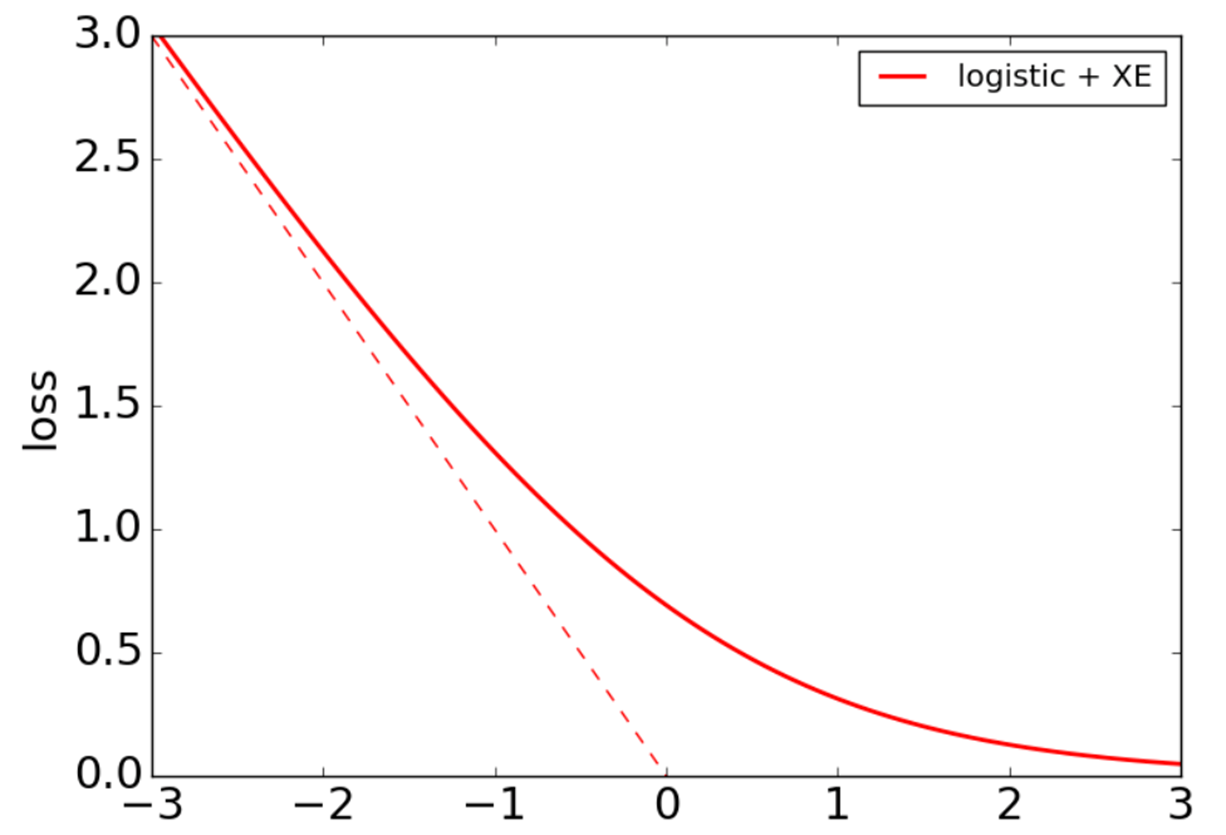
Recall the sigmiod loss.

Define the perceptron hinge loss:

$$l\left(w, x_i, y_i\right)=\max \left(0,-y_i w^T x_i\right)$$

Training process: find $w$ that minimizes (with SGD)

$$\widehat{L}(w)=\frac{1}{n} \sum_{i=1}^n l\left(w, x_i, y_i\right)=\frac{1}{n} \sum_{i=1}^n \max \left(0,-y_i w^T x_i\right)$$

The graident of perceptron loss is:

$$\nabla l\left(w, x_i, y_i\right)=-\mathbb{I}\left[y_i w^T x_i<0\right] y_i x_i$$

Support vector machine (SVM)

maximize the distance between the hyperplane
and the closest training example, where the distance is given by $\frac{\left|w^T x_0\right|}{\|w\|}$ .

finding hyperplane

Assuming the data is linearly separable, we can fix the scale of $w$ so that $y_i w^T x_i=1$ for support vectors and $y_i w^T x_i \geq 1$ for all other points.

i.e. We want to maximize margin $\frac{1}{\|w\|}$ while correctly classifying all training data: $y_i w^T x_i \geq 1$ , or

$$\min _w \frac{1}{2}\|w\|^2 \quad \text { s.t. } \quad y_i w^T x_i \geq 1 \quad \forall i.$$

Soft margin

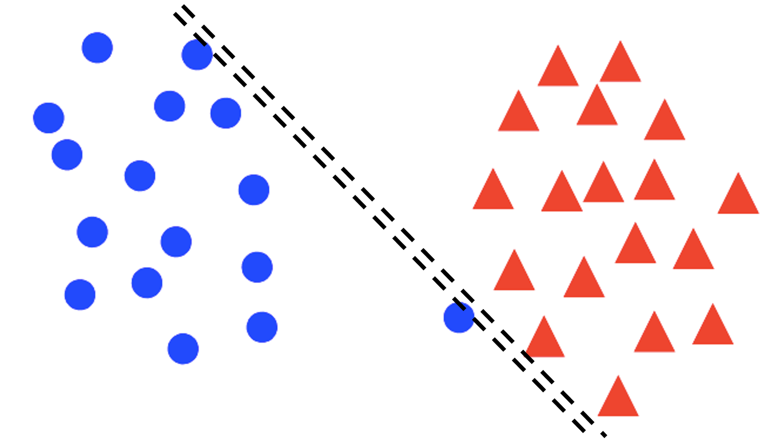
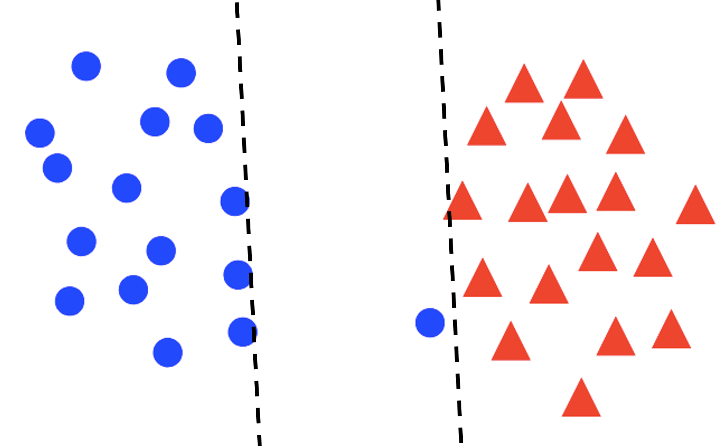
For non-separable and some separable data, we may prefer a larger margin with a few constraints violated.

$$\min _w \underbrace{\frac{\lambda}{2}\|w\|^2}_{\substack{\text { Maximize margin }- \\ \text { (regularization) }}}+\underbrace{\sum_{i=1}^n \max \left[0,1-y_i w^T x_i\right]}_{\text {Minimize misclassification loss }}$$

The loss is similar to the perceptron loss.

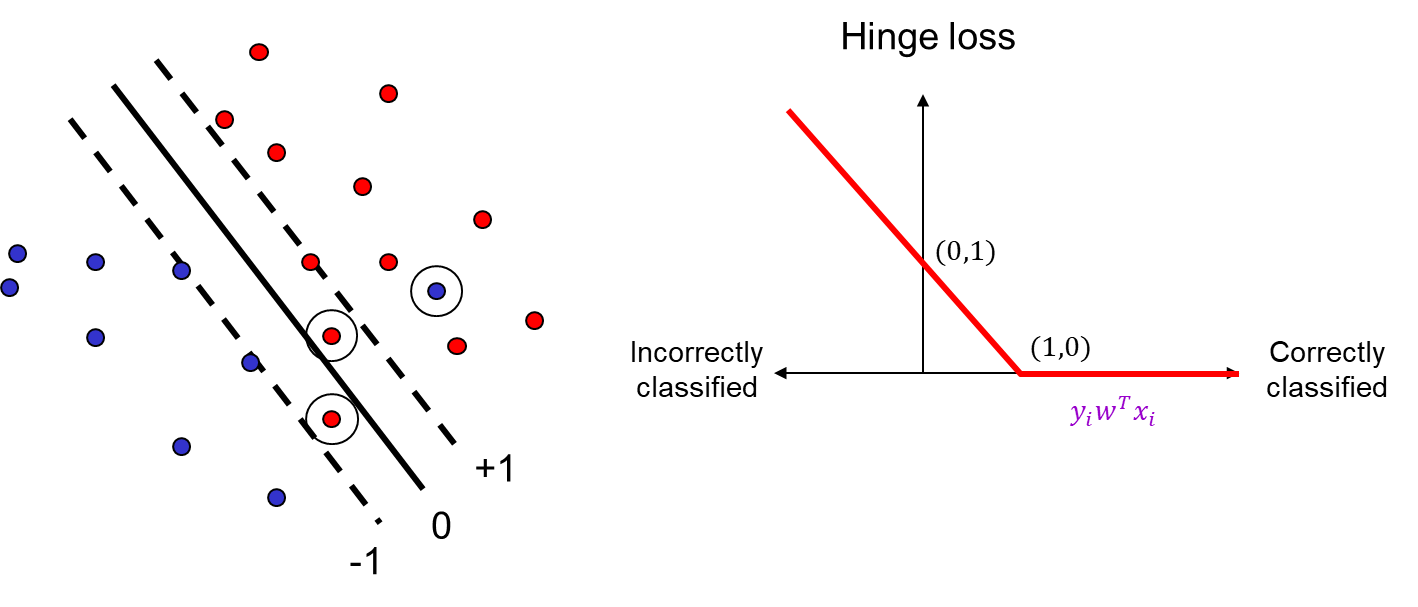
SVM and Hinge loss

This loss function tolerates wrongly classified points to get a larger margin.

SGD update

The loss function is $l\left(w, x_i, y_i\right)=\frac{\lambda}{2 n}\|w\|^2+\max \left[0,1-y_i w^T x_i\right]$ and its gradient is

$$\nabla l\left(w, x_i, y_i\right)=\frac{\lambda}{n} w-\mathbb{I}\left[y_i w^T x_i<1\right] y_i x_i.$$

General recipe

empirical loss = empirical loss + data loss

$$\hat{L}(w) \quad=\lambda R(w)+\frac{1}{n} \sum_{i=1}^n l\left(w, x_i, y_i\right)$$

regularization

• L2 regularization: $R(w)=\frac{1}{2}\|w\|_2^2$
• L1 regularization: $R(w)=\frac{1}{2}\|w\|_1 := \sum_d\left|w^{(d)}\right|$

The gradient of loss function with L1 regularization is

$$\nabla \hat{L}(w)=\lambda \operatorname{sgn}(w)+\sum_{i=1}^n \nabla l\left(w, x_i, y_i\right)$$

L1 regularization encourages sparsity weight.

Multi-class classification

Multi-class perceptron

Learn $C$ scoring functions: $f_1, f_2, \ldots, f_C$
and $\hat{y}=\operatorname{argmax}_c f_c(x)$

Multi-class perceptrons:

$$f_c(x) = w_c^T x$$

use sum of hinge losses:

$$l\left(W, x_i, y_i\right)=\sum_{c \neq y_i} \max \left[0, w_c^T x_i-w_{y_i}^T x_i\right]$$

Update rule: for each $c$ s.t. $w_c^T x_i>w_{y_i}^T x_i$ :

$$\begin{aligned} w_{y_i} & \leftarrow w_{y_i}+\eta x_i \\ w_c & \leftarrow w_c-\eta x_i \end{aligned}$$

Multi-class SVM

$$l\left(W, x_i, y_i\right)=\frac{\lambda}{2 n}\|W\|^2+\sum_{c \neq y_i} \max \left[0,1-w_{y_i}^T x_i+w_c^T x_i\right]$$

Softmax

Softmax maps a vector into probability.

$$\operatorname{softmax}\left(f_1, \ldots, f_c\right)=\left(\frac{\exp \left(f_1\right)}{\sum_j \exp \left(f_j\right)}, \ldots, \frac{\exp \left(f_C\right)}{\sum_j \exp \left(f_j\right)}\right)$$

Compared to sigmoid: for 2 class cases,

$$\operatorname{softmax}(f,-f) =(\sigma(2 f), \sigma(-2 f))$$

loss function

The negative log likelihood loss

$$l\left(W, x_i, y_i\right)=-\log P_W\left(y_i \mid x_i\right)=-\log \left(\frac{\exp \left(w_{y_i}^T x_i\right)}{\sum_j \exp \left(w_j^T x_i\right)}\right)$$

This is also the cross-entropy between the empirical distribution $\hat{P}$ and estimated distribution $P_W$ :

$$-\sum_C \hat{P}\left(c \mid x_i\right) \log P_W\left(c \mid x_i\right)$$

More on Softmax

Avoid overflow

$$\frac{\exp \left(f_c\right)}{\sum_j \exp \left(f_j\right)}=\frac{K \exp \left(f_c\right)}{\sum_j K \exp \left(f_j\right)}=\frac{\exp \left(f_c+\log K\right)}{\sum_j \exp \left(f_j+\log K\right)}$$

and let

$$\log K :=-\max _j f_j$$

Temperature

$$\operatorname{softmax}\left(f_1, \ldots, f_c ; T\right)=\left(\frac{\exp \left(f_1 / T\right)}{\sum_j \exp \left(f_j / T\right)}, \ldots, \frac{\exp \left(f_C / T\right)}{\sum_j \exp \left(f_j / T\right)}\right)$$

High temperature: close to uniform distribution.

Label smoothing

Use “Soft” prediction targets. i.e. Use empirical distribution

$$\hat{P}\left(c \mid x_i\right) = \begin{cases} 1 - \epsilon & c = y_i \\ \frac{\epsilon}{C-1} & c \neq y_i \\ \end{cases}.$$

Label smoothing is a form of regularization to avoid overly confident predictions, account for label noise