ECE313 Course Notes

De morgan

$$A^c\cap B^c = (A\cup B)^c$$

probability space $(\Omega, \mathcal{F}, P)$

$\Omega$ - sample space

$\mathcal{F}$ - collection of events

$P $- probability measure on$ \mathcal{F}$

power set denoted as $2^\Omega$

$$|2^\Omega| = 2^{|\Omega|}$$

$A, B $are mutually exclusive:$ A \cap B = \emptyset $(not$ P(A\cap B)=0$)

• example

  若样本空间是关于一个机会均等的抛硬币动作，则样本输出Ω为“正面”或“反面”。事件为：

  • {正面}，其概率为0.5。
  • {反面}，其概率为0.5。
  • { }=∅ 非正非反，其概率为0.
  • {正面，反面}，不是正面就是反面，这是Ω，其概率为1。

Axioms

event axioms

• $\Omega \in \mathcal{F}$
• $A\in \mathcal{F} \Rightarrow A^c \in \mathcal{F}$
• $A, B \in \mathcal{F} \Rightarrow A \cup B \in \mathcal{F}$
• can prove:
  • $\emptyset \in \mathcal{F}$
  • $A,B \in \mathcal{F} \Rightarrow AB \in \mathcal{F}$

probability axioms

• $P(A) \ge 0\quad \forall A \in \mathcal{F}$
• $AB = \emptyset \Rightarrow P(A\cup B) = P(A) + P(B)$
• $P(\Omega)=1$
• can prove:
  • $P(A^c) = 1 - P(A)$
  • $P(A) = P(AB) + P(AB^c)$
  • $P(A\cup B) = P(A) + P(B) - P(AB)$

Principle of counting: multiply

---

Counting

permutation - factorials

binomial coefficient

---

K map

Random Variables

for a probability space $(\Omega, \mathcal{F}, P)$

$r.v $is a real-valued function on$ \Omega$

$$X: \Omega \to \mathbb{R}$$

---

Variance and Standard Deviation

$$Var(X) := E[(X-E[X])^2] \\ \sigma_X = \sqrt{Var(X)}$$

Properties of Variance

$$Var(aX+b) = a^2Var(X)$$

$$\begin{aligned} Var(X) &= E[(X-E[X])^2] \\&=E[X^2-2XE[X]+E[X]^2] \\&=E[X^2] - 2E[X]E[X] + E[X]^2 \\&= E[X^2] - E[X]^2 \end{aligned}$$

e.g. 4 people poicking 4 card with name, expectation of # of people picking a card with their name.

$$X_i = \begin{cases}1 & choosename \\0&otherwise\end{cases}$$

then

$$X = \sum_{i=1}^4X_i$$

$$E[X] = \sum_{i=1}^4E[X_i] = \sum_{i=1}^4 \frac{1}{4}= 1$$

Variance:

because

$$X_i^2 = X_i$$

therefore

$$E[X_i^2] = \frac{1}{4}$$

$$X_iX_j = \begin{cases}1 & \text{both i,j choose their name} \\0&otherwise\end{cases}$$

and

$$E[X_iX_j] = \frac{1}{4} \frac{1}{3} = \frac{1}{12}$$

$$\begin{aligned} E[X^2] = \sum_{i=1}^4E[X_i^2]+\sum _{i\ne j}E[X_iX_j] \\ = 4 \cdot \frac{1}{4} + 12 \cdot \frac{1}{12} = 2 \end{aligned}$$

$$Var(X) = 2 - 1^2 = 1$$

Conditional Probability

Conditional Probability of B given A is defined as

$$P(B|A) = \begin{cases} \frac{P(AB)}{P(A)} &\text{if} P(A) > 0 \\ \text{undefined}\end{cases}$$

---

Independent event

$$P(B|A) = P(B)$$

Independent variable

for any $A,B \subset \mathbb{R}$ , $X \in A$ and $Y \in B$ are independent events.

this implies $P_{XY}(x,y) = P_X(x)P_Y(y)$

Properties of r.v

• independent: $E[XY]=E[X]E[Y]$
• not necessarily independent: $E[X+Y]=E[X]+E[Y]$
• independent: $Var[X+Y]=Var[X]+Var[Y]$

Bernoulli Distribution

A r.v. $X$ with range $\mathcal{X}= \{0,1\}$ ,

$$p_X(1) = p, \quad p_X(0) = 1-p$$

$$E[X] = p ,\quad Var(X) = p(1-p)$$

The Binomial Distribution

r.v. $Y$ have Bernoulli Distribution,

$n $independent experiments, each is$ Y$.

$X$ be the r.v. giving the number of ones that occur.

pmf of $X$ :

$$p_X(k) = \binom{n}{k} p^k(1-p)^{n-k}$$

$$E[X] = np, \quad Var(X) = np(1-p)$$

Geometric Distribution

Sequence of independent experiments each having a Bernoulli distribution with $p$ , $L$ is number of experiments until the outcome is 1.

$$\begin{aligned} p_L(k) & =(1-p)^{k-1} p \quad \text { for } \quad k \geq 1 . \\ P\{L>k\} & =(1-p)^k \quad \text { for } \quad k \geq 0 . \end{aligned}$$

$$E[L] = \frac{1}{p}, \quad Var(L) = \frac{1-p}{p^2}$$

Poisson Distribution

For each r.v. $X_1, X_2, \cdots$

$$C_j := \sum_{k=1}^j X_k$$

$$p(k) = \frac{\lambda ^ke^{-\lambda}}{k!}, \; \lambda = np$$

• wiki

  泊松分布 - 维基百科，自由的百科全书

$$E[Y]=\lambda,\;Var(Y)=\lambda$$

is $\lambda$ expectation or $p$ ? (in Poisson Process, $\lambda$ is $p$ )

Negative Binomial Distribution

number of failures in a sequence of independent and identically distributed Bernoulli trials before a specified (non-random) number of successes (denoted r) occurs.

$$f(k; r, p) \equiv \Pr(X = k) = \binom{k+r-1}{r-1} p^r(1-p)^k$$

$$E[k] = r \frac{1-p}{p}$$

$$Var(k) = r \frac{1-p}{p^2}$$

Maximum Likelihood Parameter Estimation

$f $is the distribution of$ x$

$$L: \theta \mapsto f(x | \theta) \\ \hat{\theta}_{\mathrm{ML}}(x) = \argmax_{\theta} f(x | \theta)$$

---

Markov inequality

if $Y$ is a nonnegative random variable, the for $c>0$ ,

$$Pr\{Y\ge c\} \le \frac{E[Y]}{c}$$

Proof.

$$\begin{aligned}\textrm{E}(X) &= \int_{-\infty}^{\infty}x f(x) dx \\&= \int_{0}^{\infty}x f(x) dx \\[6pt]&\geqslant \int_{a}^{\infty}x f(x) dx \\[6pt]&\geqslant \int_{a}^{\infty}a f(x) dx \\[6pt]&= a\int_{a}^{\infty} f(x) dx \\[6pt]&=a\textrm{P}(X\geqslant a).\end{aligned}$$

Chebyshev’s Inequality

$$\Pr(|X-\textrm{E}(X)| \geq a) \leq \frac{\textrm{Var}(X)}{a^2}$$

Proof.

$$\operatorname{Var}(X) = \operatorname{E}[(X - \operatorname{E}(X) )^2].$$

use Markov inequality,

$$\Pr( (X - \operatorname{E}(X))^2 \ge a^2) \le \frac{\operatorname{Var}(X)}{a^2},$$

Confidence Interval

With r.v. $\hat p = \frac{X}{n}$ (sampling) and $\mu = E[\hat p] = p$ (real p)

then

$$Var(\hat p) = \frac{Var(X)}{n} = \frac{p(1-p)}{n}$$

and`

$$\begin{array}{c}\operatorname{Pr}\left\{\left|\hat{p}^{}-\mu\right|<\sigma b\right\}>1-\frac{1}{b^{2}} \\\Rightarrow \operatorname{Pr}\{\mu \in(\hat{p}-\sigma b, \hat{p}+\sigma b)\}>1-\frac{1}{b^{2}} \\\Rightarrow \operatorname{Pr}\left\{p \in\left(\hat{p}-b \sqrt{\frac{p(1-p)}{n}}, \hat{p}+b \sqrt{\frac{p(1-p)}{n}}\right)\right\}>1-\frac{1}{b^{2}}\end{array}$$

Use bound $\sqrt{p(1-p)} \le \frac{1}{2}$  ,

$$\operatorname{Pr}\left\{p \in\left(\hat{p}-\frac{b}{2 \sqrt{n}}, \hat{p}+\frac{b}{2 \sqrt{n}}\right)\right\}>1-\frac{1}{b^{2}}$$

$1-\frac{1}{b^2} $is confidence level,$ \frac{b}{2 \sqrt{n}}$ is confidence width,

---

Conditional mean

$$E[X|A] = \sum_i u_iP(X=u_i|A)$$

LOTUS (Law of the unconscious statistician)

$$E[g(X)|A] = \sum_i g(u_i)P(X=u_i|A)$$

Total Probability Theroem

$$P(B) = \sum_i{P(A_iB)} \\P(B) = \sum_i{P(B|A_i)P(A_i)}$$

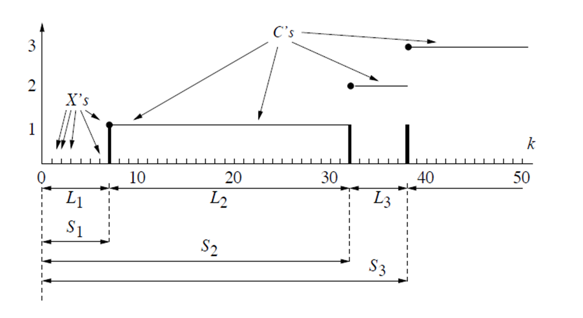
Response of Stochastic System

Bayes’ theorem

$$P(A|B) = \frac{P(B|A)P(A)}{P(B)} =\frac{P(A_i)P(B|A_i)}{\sum_iP(B|A_i)P(A_i)}$$

MAP v.s ML

ML

$$L:\theta \mapsto P(x|\theta) \\ \hat \theta =\argmax_\theta P(x|\theta)$$

MAP

$$L:\theta \mapsto P(\theta|x) \\ \hat \theta =\argmax_\theta P(\theta|x) = \argmax_\theta \frac{P(x|\theta)P(\theta)}{\sum_{\theta'}P(x|\theta')g(\theta ')}$$

---

Network Probability

edge i has a probability $p_i$ of failing

Boole’s Inequality (Union Bound)

$$P\left(\bigcup_{i} A_i\right) \le \sum_i P(A_i)$$

---

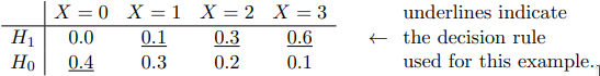
Binary hypothesis testing with discrete-type observations

Likelihood matrix

Either hypothesis $H_0$ or $H_1$ is true. If $H_0$ is true, $X$ has a pmf $p_0$ , if $H_0$ is true, $X$ has a pmf $p_0$ , as showed in the Likelihood matrix.

Decision rule

As mentioned above, a decision rule specifies, for each possible observation, which hypothesis is declared.

• false alarm: $H_0$ is true, $H_1$ is declared.
• miss: $H_1$ is true, $H_0$ is declared.

$$p_{\text{false alarm} } = P(\text{declare} H_1 \text{true} | H_0) \\ p_{\text{miss} } = P(\text{declare} H_0 \text{true} | H_1)$$

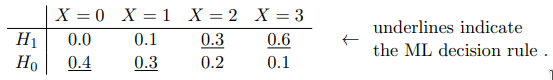
Maximum likelihood (ML) decision rule

ML decision rule

another way: likelihood ratio test (LRT)

Define the likelihood ratio

$$\Lambda(k) = \frac{p_1(k)}{p_0(k)}$$

$$\Lambda(X) \begin{cases}>1 & \text { declare } H_1 \text { is true } \\ <1 & \text { declare } H_0 \text { is true. }\end{cases}$$

or

$$\Lambda(X) \begin{cases}>\tau & \text { declare } H_1 \text { is true } \\ <\tau & \text { declare } H_0 \text { is true }\end{cases}$$

ML decision rule is $\tau = 1$ .

• increase $\tau$ : miss
• decrease $\tau$ : false alarm

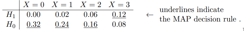
Maximum a posteriori probability (MAP) decision rule

make use of $P(H_0)$ and $P(H_0)$ prior knowledge and use joint probability such as $P(\{X=1\}\cap H_1)$ .

denote

$$P(H_0) = \pi_i$$

the joint probabilities are

$$P(H_i, X=k) = \pi_ip_i(k)$$

joint probability matrix $\pi_0 = 0.8, \pi_1 = 0.2$

equivalent to

$$\tau = \frac{\pi_0}{\pi_1}$$

‘uniform’ means $\pi_0 = \pi_1$

average error probability $p_e$

$$p_{e}=\pi_{0} p_{\text {false alarm }}+\pi_{1} p_{\text {miss }}$$

minimize $p_e$ $\iff$ maximize:

$$\begin{aligned}& \pi_0 P(\text{declare} H_0|H_0) + \pi_1 P(\text{declare} H_1|H_1) \\=&\sum_k \pi_0 P(X=k|H_0)P(\text{declare} H_0|X=k) + \\&\pi_1 P(X=k|H_1)P(\text{declare} H_1|X=k) \\\end{aligned}$$

, therefore,

$$i_{\text{declare} } = \argmax_i \;\pi_i P(X=k|H_i)$$

So MAP decision rule is the one that minimizes $p_e$ . The MAP rule is also called the minimum
probability of error rule.

---

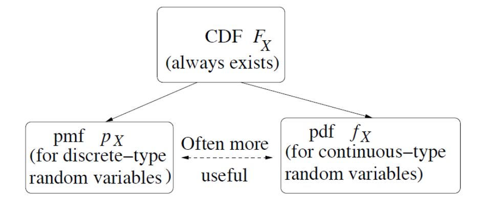
cdf

what to do if $\Omega$ is uncountable?

the usual event algebra in this case if the Borel algebra.

it is the smallest algebra closed under formation of countably many unions and intersections containing all finite intervals in $\mathbb{R}$

$$\epsilon = (\mathbb{R}, \mathcal{B}, P)$$

$$F_X(C) = \operatorname{Pr}(X\le C)$$

$F_X $determines probability measure on semi-infinite intervals$ \rightarrow$ suffices determines all intervals.

Size of jump points of cdf:

$$\Delta F_X(x) = F_X(c) -F_X(c-)$$

$$P(X \in (a,b]) = F_X(b) - F_X(a), \quad a < b$$

$$P(X < c) = F_X(c-)$$

$$P(X = c) = \Delta F_X(c)$$

---

pdf

$$1 = \int_{-\infty}^{+\infty}f_X(u)du$$

$$E[X] = \int_{-\infty }^{\infty }u f_X(u)du$$

$$E[X^2] = \int_{-\infty }^{\infty }u^2 f_X(u)du$$

$$\operatorname{Var}(X) = E[X^2] - E[X]$$

---

if continuous at $c$

$$F_X'(c) = f_X(c)$$

The Exponential Distribution

cdf

$$F_{X}(t)=\left\{\begin{array}{ll}1-e^{-\lambda t} & t \geq 0 \\0 & t<0\end{array}\right.$$

pdf

$$f_{X}(t)=\left\{\begin{array}{l}\lambda e^{-\lambda t} \quad t \geq 0 \\0 \quad t<0\end{array}\right.$$

$$E[X] = \frac{1}{\lambda} \\ E[X^n] = \frac{n!}{\lambda^n}$$

$$Var(X) = \frac{1}{\lambda^2}$$

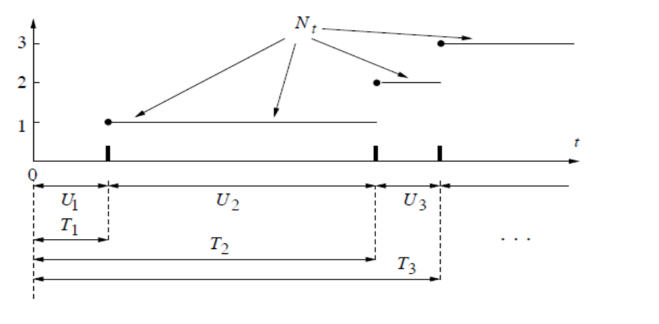
The Poisson process

泊松过程 - 维基百科，自由的百科全书

Different distribution in one graph

$N_t$ are counting variables

$$P\left\{N_{t}=k\right\}=\frac{[\lambda t]^{k}}{k !} e^{-\lambda t}$$

$U_i$ are delay variables

have Exponential Distributions

$$f_{U_{i}}(t)=\left\{\begin{array}{l}\lambda e^{-\lambda t} \quad t \geq 0 \\0 \quad t<0\end{array}\right.$$

$T_k$ are time variables

$$T_r = \sum_{i=1}^r U_i$$

have Erlang Distributions

---

The Erlang Distribution

In a Poisson process with arrival rate $\lambda$ , the time that $k$ -th events happens is Erlang Distribution.

$$f(x; k,\lambda)={\lambda^k x^{k-1} e^{-\lambda x} \over (k-1)!}\quad{\text{for }}x, \lambda \geq 0$$

Linear Scaling of pdfs

$$Y = aX+b$$

is a linear transformation of $X$

cdf:

$$F_Y(y) = F_X(\frac{y-b}{a} )$$

pdf

$$f_Y(y) = \frac{dF_Y(y)}{dy} = \frac{1}{a}f_X(\frac{y-b}{a} )$$

---

The Uniform Distribution

$$X \sim \mathcal{U}_{[a,b]} \\ Var(X) = \frac{1}{12}(b-a)^2 \\ E[X] = \frac{a+b}{2}$$

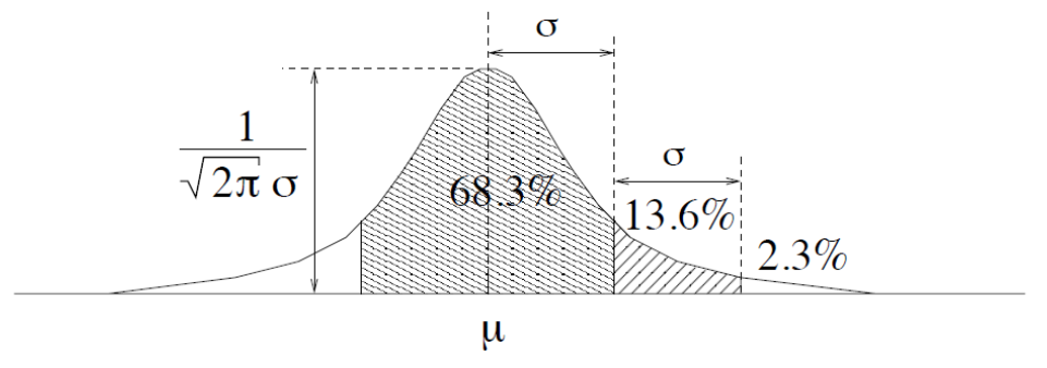
The Gaussian (Normal) Distribution

$N(\mu,\sigma^2)$:

$$f(x)=\frac{1}{\sqrt{2 \pi \sigma^{2}}} \exp \left(-\frac{(x-\mu)^{2}}{2 \sigma^{2}}\right)$$

pdf

$$f(x) = \frac{1}{\sqrt{2\pi}}\exp\left(-\frac{x^2}{2}\right)$$

cdf

$$\Phi(x) = \frac{1}{\sqrt{2\pi}} \int_{-\infty}^{x}\exp\left(-\frac{u^2}{2}\right) du$$

$$Q(x) = P(S>x)=1-\Phi(x)$$

$N(\mu,\sigma^2) $can be obtained from the standard distribution$ Y=\sigma X+\mu$.

$$E[Y] = E[\sigma X+\mu] = \mu$$

$$Var(Y) = Var(\sigma X+\mu) = \sigma^2$$

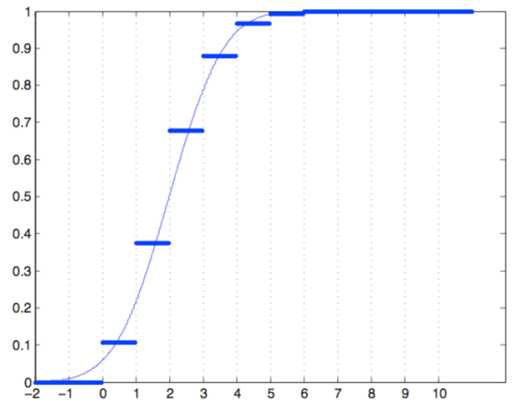
The Central Limit Theorem

Let $S_{n,p} \sim \operatorname{Bin}(n,p)$ , and standardized version:

$$\hat S_{n,p} := \frac{S_{n,p} - \mu}{\sigma}$$

then

$$\lim _{n \rightarrow \infty} P\left\{\hat{S}_{n, p} \leq c\right\}=\Phi(c)$$

The Central Limit Thm Continuity Correction

when bounded from above

$$\begin{aligned} P\left\{S_{n, p} \leq L\right\} \rightarrow &P\left\{S_{n, p}-\frac{1}{2} \leq L\right\} \\ =&P\left\{\frac{S_{n, p}-\mu-\frac{1}{2}}{\sigma} \leq \frac{L-\mu}{\sigma}\right\} \\ =&P\left\{\hat{S}_{n, p} \leq \frac{L-\mu+\frac{1}{2}}{\sigma}\right\} \\ \approx &\Phi\left(\frac{L-\mu+\frac{1}{2}}{\sigma}\right) . \end{aligned}$$

when bounded from below

$$P\left\{S_{n, p} \geq L\right\} \rightarrow P\left\{S_{n, p}+\frac{1}{2} \geq L\right\}$$

---

Generating a r.v. with a specified distribution

$U $is r.v. **uniformly** distributed on$ [0,1] $, find$ g $such that$ g(U) $has a distribution$ F$.

Let $g(u) = F^{-1}(u)$ ,

then let $X=g(U)$ , then

$$F_X(g(u))=F_U(u)=u$$

suffices.

Failure Rate Functions

For r.v. $T$ describing a lifetime of a system, the failure rate function is:

$$h(t) = \lim_{\epsilon \to 0}\frac{P\{t<T<t + \epsilon |T>t\}}{\epsilon }$$

then, given that the system is not failed up to time $t$ , the probability that is will fail within the next $\epsilon$ -time interval is

$$T \in (t,t+\epsilon ) \sim  h(t)\epsilon$$

the $h(t)$ can be expressed as

$$\begin{aligned}h(t):=\lim _{\epsilon \rightarrow 0} \frac{P\{t<T<t+\epsilon \mid T>t\}}{\epsilon} & =\lim _{\epsilon \rightarrow 0} \frac{P\{t<T<t+\epsilon\}}{\epsilon P\{T>t\}} \\& =\lim _{\epsilon \rightarrow 0} \frac{F_{T}(t+\epsilon)-F_{T}(t)}{\epsilon\left(1-F_{T}(t)\right)} \\& =\frac{F_{T}^{\prime}(t)}{1-F_{T}(t)}=\frac{f_{T}(t)}{1-F_{T}(t)} .\end{aligned}$$

notice that

$$-h(t)=[\ln(1-F_T(t))]' \\ -\int_0^th(t)dt=\ln(1-F_T(t))-\ln(1-F_T(0))=\ln(1-F_T(t)) \\ \text{therefore, } F_T(t) = 1-\exp\left(-\int_0^t h(t) dt\right).$$

Hypothesis Testing

see also: Binary hypothesis testing with discrete-type observations

A random variable $X$ has pdf $f_1$ (hypothesis $H_1$ ) or $f_0$ (hypothesis $H_0$ ).

For observation $u$ , form the likelihood ratio of pdfs:

$$\Lambda(u) = \frac{f_1(u)}{f_0(u)}$$

ML rule

$$\begin{cases}\Lambda(u) > 1 & \text{declare } H_1 \\\Lambda(u) < 1 & \text{declare } H_0\\\end{cases}$$

MAP rule

with prior probabilities $\pi_0$ and $\pi_1$ ,

$$\begin{cases}\Lambda(u) > \frac{\pi_0}{\pi_1}  & \text{declare } H_1 \\\Lambda(u) < \frac{\pi_0}{\pi_1} & \text{declare } H_0\\\end{cases}$$

error

$$p_{e}=P\left(\text { Declare } H_{1} \mid H_{0}\right) \pi_{0}+P\left(\text { Declare } H_{1} \mid H_{1}\right) \pi_{1}$$

Jointly Distributed Random Variables

joint CDF

$$F_{XY}(u, v) = P\{X\le u, Y\le v\}.$$

$$P\{(X, Y) \in (a,b]\times (c,d]\}=F_{X, Y}(b, d)-F_{X, Y}(a, d)-F_{X, Y}(b, c)+F_{X, Y}(a, c) .$$

Is a functon valid joint CDF?

To be a valid joint CDF for two random variables $U$ and $V$ , a function must satisfy several properties:

1. Non-decreasing: $F(u, v)$ must be non-decreasing in both $u$ and $v$ . That is, if $u_1 \leq u_2$ and $v_1 \leq v_2$ , then $F(u_1, v_1) \leq F(u_2, v_2)$ .

2. Right-continuous: $F(u, v)$ must be right-continuous in both $u$ and $v$ .

3. Limits at infinity:

   • $\lim_{u \to -\infty} F(u, v) = 0$ for all $v$
   • $\lim_{v \to -\infty} F(u, v) = 0$ for all $u$
   • $\lim_{u \to \infty} F(u, v) = F(\infty, v)$ for all $v$
   • $\lim_{v \to \infty} F(u, v) = F(u, \infty)$ for all $u$
   • $\lim_{u \to \infty, v \to \infty} F(u, v) = 1$

4. Non-negativity: $F(u, v) \geq 0$ for all $u, v$ .

5. Joint Probability: For any $u_1 < u_2$ and $v_1 < v_2$ , the joint probability should be non-negative:
   $F(u_2, v_2) - F(u_2, v_1) - F(u_1, v_2) + F(u_1, v_1) \geq 0$

Joint PMF

$$p_{XY}(x,y) = \{X=x, Y=y\}$$

Marginal pdf

$$f_X(x)=\int_{-\infty}^{\infty}f_{XY}(x,y)dy$$

The Marginal cdfs

$$F_{X}(u)=\lim _{n \rightarrow \infty} F_{X, Y}(u, n) \quad \text { and } \quad F_{Y}(v)=\lim _{n \rightarrow \infty} F_{X, Y}(n, v)$$

The Conditional pdf

$$f_{Y|X}(v|u) = \begin{cases}\frac{f_{XY}(u,v)}{f_X(u)} & \text{if} f_X(u)\ne 0 \\\text{undefined} &  \text{if} f_X(u) = 0 \\\end{cases}$$

$$E[Y|X=u] = \int_{-\infty}^{\infty}yf_{Y|X}(y|x)dy$$

Sum or r.v

given $Z = X + Y$

$$E[Z]=E[X]+E[Y]$$

$$Var(Z) = Var(X) + Var(Y) + 2 Cov(X, Y) \\ Var(X-Y) = Var(X) + Var(Y) - 2 Cov(X, Y) \\$$

$$Cov(X,Y)=E[(X−E[X])(Y−E[Y])]$$

If X and Y are independent, then $Cov(X, Y) = 0$ .

$$\begin{array}{c}p_{Z}(u)=p_{X}(u) * p_{Y}(u) \\p_{Z}(u)=\sum_{k=-\infty}^{\infty} p_{X}(k) p_{Y}(u-k)=\sum_{k=-\infty}^{\infty} p_{X}(u-k) p_{Y} (k) \\\end{array}$$

$$\begin{array}{c}f_{Z}(u)=f_{X}(u) * f_{Y}(u) \\f_{Z}(u)=\int_{-\infty}^{\infty} f_{X}(\tau) f_{Y}(u-\tau) d \tau=\int_{-\infty}^{\infty} f_{X}(u-\tau) f_{Y}(\tau) d \tau\end{array}$$

Linear Transformation of Joint R.V.s

$$(X, Y) \mapsto(W, Z) \quad \text { where } \quad \begin{array}{c} W = aX+b Y \\ Z = c X+d Y \end{array}$$

$$\begin{pmatrix} W \\ Z \end{pmatrix} = A \begin{pmatrix} X \\ Y \end{pmatrix} \quad \text{where} \quad Z = \begin{pmatrix} a & b \\ c & d \end{pmatrix}$$

Proposition

$$f_{W Z}(w, z)=\frac{1}{|\operatorname{det} A|} f_{X Y}\left(A^{-1}\left(\begin{array}{c} w \\ z \end{array}\right)\right)$$

Correlation and Covariance

For r.v. $X$ , $Y$

correlation

$$E[XY]$$

covirance

$$Cov(X, Y) := E[(X-E[X])(Y-E[Y])]$$

$$Cov(X, Y) = E[XY]- E[X]E[Y] \\ Cov(X, X) = Var(X)$$

correlation coeffcient

$$\rho_{X Y}=\frac{\operatorname{Cov}(X, Y)}{\sqrt{\operatorname{Var}(X)} \sqrt{\operatorname{Var}(Y)}}=\frac{\operatorname{Cov}(X, Y)}{\sigma_X \sigma_Y}$$

if $E[X] = E[Y] = 0$

$$Cov(X, Y) = E[XY]$$

$X $,$ Y$ are uncorelated if

$$Cov(X, Y) = 0$$

$X $,$ Y$ are positively corelated if

$$Cov(X, Y) > 0$$

and

$$Cov(X+Y, U+V) = Cov(X, U) + Cov(X, V) + Cov(Y, U) + Cov(Y, V)$$

$$Cov(aX+b, cY+d) = acCov(X, Y)$$

Cauchy-Schwarz Inequality

$$|E[X Y]| \leq \sqrt{E\left[X^2\right] E\left[Y^2\right]}$$

$$|\operatorname{Cov}(X, Y)| \leq \sqrt{\operatorname{Var}(X) \operatorname{Var}(Y)}$$

Minimum Mean Square Error Estimation

flowchart LR
    A[Experiment] -->|Y| B[Noise]
    B -->|X| C[Guess]
    C -->|"g(X)=Y"| ...

An estimator is unbiased if

$$E[\hat{T}] = E[Y]$$

Constant estimators

(Continued) To minimize MSE with Constant estimator $\delta$ ,

$$\begin{aligned} E\left[(Y-\delta)^2\right] & = E\left[Y^2\right]-2 \delta E[Y]+\delta^2 \\ & = E[Y^2] - E[Y]^2 + E[Y]^2 - 2\delta E[Y] + \delta^2 \\ & = Var(Y) + (E[Y]-\delta)^2 \end{aligned}$$

therefore, MSE is minimized iff $\delta = E[Y]$ and minimum MSE is $Var(Y)$ .

Unconstrained estimators

We wish to estimate $Y$ based on an observation $X$ .

Goal: Minimize the mean-square error (MSE)

$$E[(Y-g(X))^2]$$

The resulting estimator $g^*(X)$ is called the unconstrained optimal
estimator of $Y$ based on $X$ (because no constraints are placed on the function $g$ ).

For a observation $X=u$ , similar to Constant estimators,

$$g^*(u)=E[Y \mid X=u]=\int_{-\infty}^{\infty} v f_{Y \mid X}(v \mid u) d v$$

and

$$\begin{aligned} MSE & = E[(Y-E[Y|X])^2] \\ &= E[Y^2] - E[(E[Y|X])^2] \\ &= E[Y^2] - E[g^*(X)^2] \end{aligned}$$

Linear estimators

Because $E[Y| X=u]=\int_{-\infty}^{\infty} v f_{Y | X}(v | u) d v$ may be diffcult, use a linear estimator

$$L(X) = aX + b$$

as $g(X)$ .

With a given $a$ . the optimal linear estimator is

$$\mu_Y + a(X-\mu_X)$$

then

$$\begin{aligned} M S E & =E\left[\left(Y-\mu_Y-a\left(X-\mu_X\right)\right)^2\right] \\ & =\operatorname{Var}(Y-a X) \\ & =\operatorname{Cov}(Y-a X, Y-a X) \\ & =\operatorname{Var}(Y)-2 a \operatorname{Cov}(Y, X)+a^2 \operatorname{Var}(X) . \end{aligned}$$

To minimize $MSE$ , take $0 = \frac{d}{da}MSE$ , get

$$a^* = \frac{Cov(Y,X)}{Var(X)}$$

i.e.

$$\begin{aligned} L^*(X) & =\mu_Y+\left(\frac{\operatorname{Cov}(Y, X)}{\operatorname{Var}(X)}\right)\left(X-\mu_X\right) \\ & =\mu_Y+\sigma_Y \rho_{X, Y}\left(\frac{X-\mu_X}{\sigma_X}\right) . \end{aligned}$$

and minimum MSE is

$$\sigma_Y^2-\frac{\operatorname{Cov}(X, Y)^2}{\operatorname{Var}(X)}=\sigma_Y^2\left(1-\rho_{X, Y}^2\right)$$

Odering

$$\underbrace{E\left[\left(Y-g^*(X)\right)^2\right]}_{\text {MSE for } g^*(X)=E[Y \mid X]} \leq \underbrace{\sigma_Y^2\left(1-\rho_{X, Y}^2\right)}_{\text {MSE for } L^*(X)=\widehat{E}[Y \mid X]} \leq \underbrace{\sigma_Y^2}_{\text {MSE for } \delta^*=E[Y] .}$$

for joint Gaussian, $g^*(X)=L^*(X)$

Law of Large Numbers

recall Chebyshev’s Inequality

Let $X_1, X_2, \cdots X_n$ independent r.v.'s, each having same mean $\mu$ and variance $Var(X)=\sigma^2$ , consider the sample mean:

$$\overline{X_n} = \frac{1}{n} \sum_{k=1}^{n} X_k$$

Law of Large Numbers

for any $s>0$ ,

$$P\left\{ |\overline{X_n} - \mu| \ge s \right\} \le \frac{\sigma^2}{ns^2} \to 0$$

Central Limit Theorem

Let

$$Z_n=\frac{\overline{X_n}-\mu}{\frac{\sigma}{\sqrt{n}}}$$

then $E[Z_n] = 0$ and $Var(Z) = 1$ , and $Z_n$ converges to a statndard Gaussian Distribution.

$$\lim_{n\to \infty} F_{Z_n} (c) = \Phi(c)$$

The Central Limit Theorem Continuity Correction

• Replace $\sum_{i=1}^n X_i \rightarrow \sum_{i=1}^n X_i-\frac{1}{2}$ when bounded from above.
• Replace $\sum_{i=1}^n X_i \rightarrow \sum_{i=1}^n X_i+\frac{1}{2}$ when bounded from below.

$$P\left\{\sum_{i=1}^n X_i \leq L\right\} \to P\left\{\sum_{i=1}^n X_i-\frac{1}{2} \leq L\right\} \\=P\left\{Z_n \leq \frac{L-n \mu+\frac{1}{2}}{\sqrt{n} \sigma}\right\} \approx \Phi\left(\frac{L-n \mu+\frac{1}{2}}{\sqrt{n} \sigma}\right)$$

$$P\left\{\sum_{i=1}^n X_i \geq L\right\} \to P\left\{\sum_{i=1}^n X_i+\frac{1}{2} \geq L\right\} \\=P\left\{Z_n \geq \frac{L-n \mu-\frac{1}{2}}{\sqrt{n} \sigma}\right\} \approx 1 - \Phi\left(\frac{L-n \mu-\frac{1}{2}}{\sqrt{n} \sigma}\right)$$

Joint Gaussian Random Variables

sum of Joint Gaussian Random Variables are also Gaussian Random Variables.

$$f_{W Z}(w, z)=f_W(w) f_Z(z)=\frac{1}{2 \pi} \exp \left(-\frac{w ^2+z^2}{2}\right)$$

Linear Transformation of Joint R.V.s

$$(W,Z) \mapsto (X, Y) \\ \begin{pmatrix} X \\ Y \end{pmatrix} = A \begin{pmatrix} W \\ Z \end{pmatrix}+\bold{b} \quad \text{where}\; A= \begin{pmatrix} a & b\\ c & d \end{pmatrix}$$

$$\begin{pmatrix} W \\ Z \end{pmatrix} = A^{-1} \begin{pmatrix} X \\ Y \end{pmatrix} \quad \text{where}\; A^{-1}= \frac{1}{\det{A}} \begin{pmatrix} d & -b\\ -c & a \end{pmatrix}$$

Proposition: If $A$ is invertible, then

$$f_{X Y}(x, y)=\frac{1}{|\det A|} f_{W Z}\left(A^{-1}\left(\begin{array}{l} x \\ y \end{array}\right)\right) .$$

Let $\sigma_X > 0,\, \sigma_Y > 0,\, \mu_X,\, \mu_Y,\, -1<\rho<1$ , then linear transformation

$$A=\left(\begin{array}{cc} \sigma_X \sqrt{(1+\rho) / 2} & -\sigma_X \sqrt{(1-\rho) / 2} \\ \sigma_Y \sqrt{(1+\rho) / 2} & \sigma_Y \sqrt{(1-\rho) / 2} \end{array}\right) \quad b=\left(\begin{array}{c} \mu_X \\ \mu_Y \end{array}\right)$$

then $\left(\begin{array}{c} W \\ Z \end{array}\right) \rightarrow\left(\begin{array}{l} X \\ Y \end{array}\right)=A\left(\begin{array}{c} W \\ Z \end{array}\right)+b$ gives a bivariate Gaussian pdf:

$$f_{X Y}(x, y)=\frac{1}{2 \pi \sigma_X \sigma_Y \sqrt{1-\rho^2}} \exp{-\frac{\left(\frac{x-\mu_X}{\sigma_X}\right)^2+\left(\frac{y-\mu_Y}{\sigma_Y}\right)^2-2 \rho\left(\frac{x-\mu_X}{\sigma_X}\right)\left(\frac{y-\mu_Y}{\sigma_Y}\right)}{2\left(1-\rho^2\right)}}$$

Or, with normalized $\tilde{x} = \frac{x-\mu_x}{\sigma_x},\; \tilde{y} = \frac{y-\mu_y}{\sigma_y}$ :

$$f_{X Y}(x, y)=\frac{1}{2 \pi \sigma_X \sigma_Y \sqrt{1-\rho^2}} \exp{-\frac{(\tilde{y}-\rho \tilde{x})^2}{2\left(1-\rho^2\right)}} \exp -\frac{x^2}{2}$$

Properties

$$f_X(x) = \int_{-\infty}^{+\infty} dyf_{XY}(x, y) \\=\frac{1}{\sqrt{2 \pi \sigma_x^{2}}} \exp \left(-\frac{(x-\mu_x)^{2}}{2 \sigma_x^{2}}\right)$$

$$f_{Y \mid X}(y \mid x)=\frac{1}{\sqrt{2 \pi} \sigma_Y \sqrt{1-\rho^2}} \exp{-\frac{1}{2} \frac{\left(y-\mu_Y-\rho \sigma_Y\left(x-\mu_X\right) / \sigma_X\right)^2}{\sigma_Y^2\left(1-\rho^2\right)}} \\ =N\left(\mu_Y+\rho \sigma_Y\left(\frac{x-\mu_X}{\sigma_X}\right), \sigma_Y^2\left(1-\rho^2\right)\right) \\ = N\left(E[Y|X=x], \sqrt{Var(Y|X=x)}\right)$$

Or, normalized:

$$f_{Y \mid X}(y \mid x)=\frac{1}{\sqrt{2 \pi} \sqrt{1-\rho^2}} e^{-\frac{1}{2} \frac{(y-\rho x)^2}{1-\rho^2}} \\ = N(\rho x, 1 - \rho^2)$$

Unconstrained estimator $g$

$$g^*(x) = L^*(x)=E[Y|X=x]=\mu_Y + \rho\sigma_Y\left(\frac{x-\mu_X}{\sigma_X}\right)$$