The basic supervised learning framework
y=f(x)
- y : output
- f : prediction function
- x : input
training:
(x1,y1),…,(xN,YN)
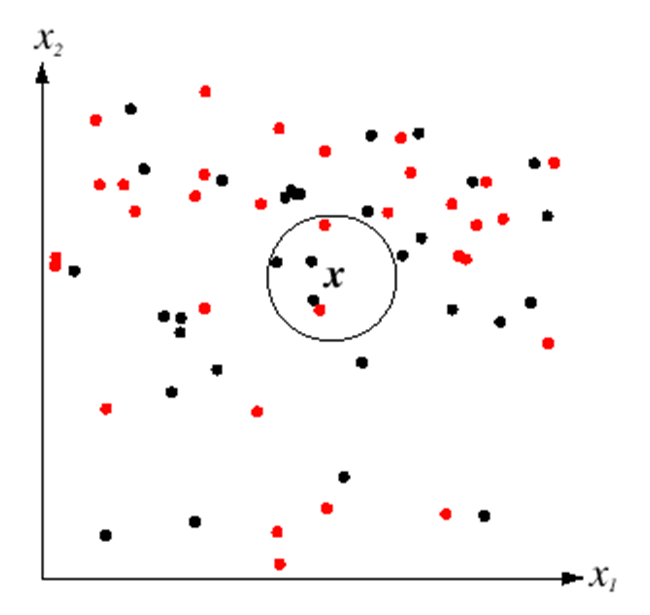
Nearest neighbor classifier
$f(x) =labelofthetrainingexamplenearestto x$
K-nearest neighbor classifier:

Linear classifier
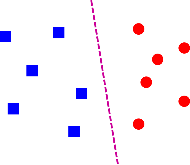
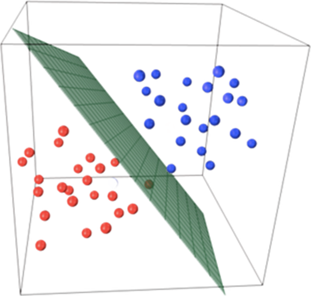
f(x)=sgn(w⋅x+b)
NN vs. linear classifiers: Pros and cons
NN pros:
- Simple to implement
- Decision boundaries not necessarily linear
- Works for any number of classes
- Nonparametric method
NN cons:
- Need good distance function
- Slow at test time
Linear pros:
- Low-dimensional parametric representation
- Very fast at test time
Linear cons:
- Works for two classes
- How to train the linear function?
- What if data is not linearly separable?
Empirical loss minimization
define expected loss
L(f)=E(x,y)∼D[l(f,x,y)]
- 0−1 loss
- l(f,x,y)=I[f(x)=y]
- L(f)=Pr[f(x)=y]
- l2 loss
- l(f,x,y)=[f(x)−y]2
- L(f)=E[[f(x)−y]2]
Find f that minimizes
L^(f)=n1i=1∑nl(f,xi,yi)
- for 0−1 loss
- NP-hard
- use surrogate loss functions instead
- l2 loss
- L^(fw)=n1∥Xw−Y∥2 is a convex function
- 0=∇∥Xw−Y∥2=2XT(Xw−Y)
- w=(XTX)−1XTY
Interpretation of l2 loss
Assumption:
$y isnormallydistributedwithmean f_w(x) = w^Tx+b$
Maximum likelihood estimation:
wML=wargmin−i∑logPw(yi∣xi)=wargmini∑−log(2πσ21exp(−2σ2[yi−fw(xi)]2))=wargmini∑log2πσ2+2σ2[yi−fw(xi)]2=wargmini∑[yi−fw(xi)]2
Problem of linear regression

Linear regression is very sensitive to outliers
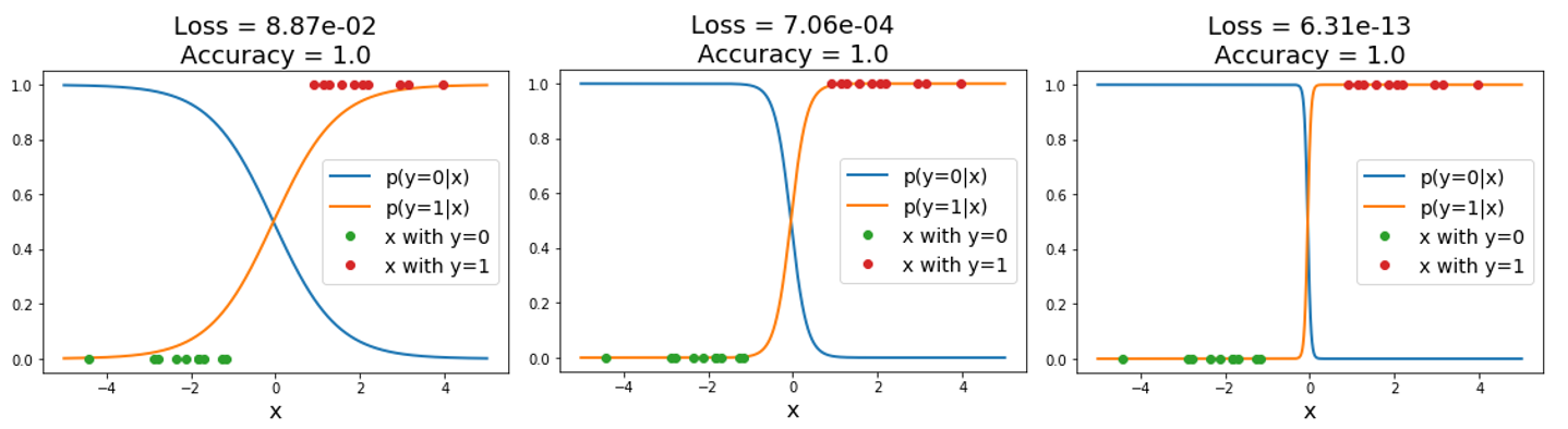
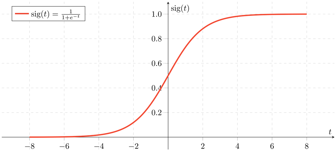
Logistic regression
use sigmoid function
σ(x)=1+e−x1
flowchart LR
    x,y-->linear_output
    linear_output-->|logistic function|Probability
sigmoid function
Pw(y=1∣x)=σ(wTx)=1+exp(−wTx)1
Pw(y=−1∣x)=1−Pw(y=1∣x)=σ(−wTx)
logP(y=−1∣x)P(y=1∣x)=wTx+b
Logistic loss
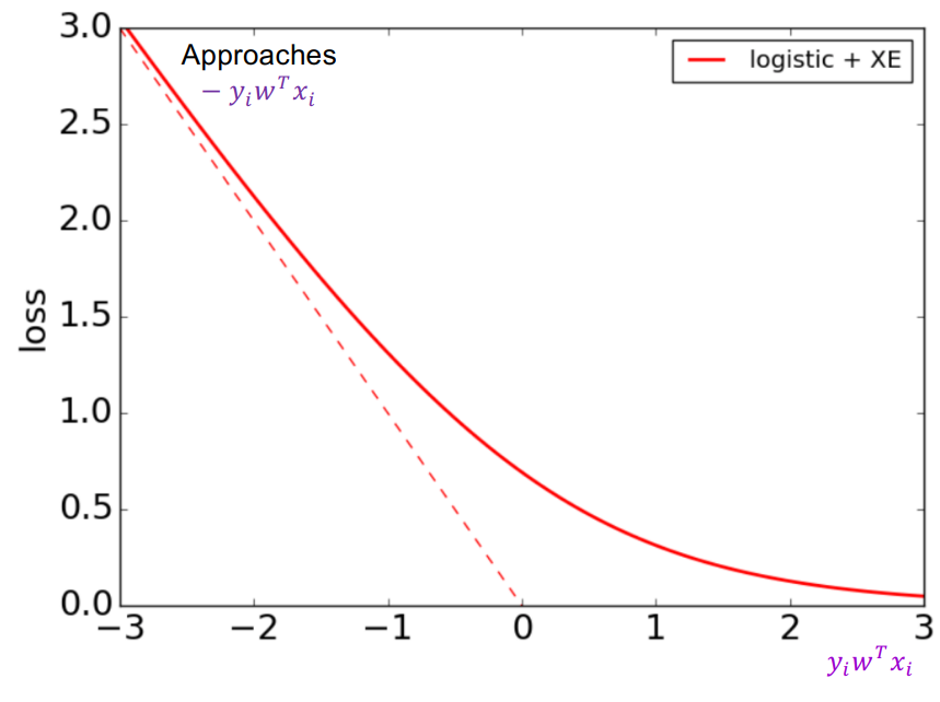
Maximum likelihood estimate:
wML=wargmini∑−logP(yi∣xi)=wargmini∑−logσ(yiwTxi)
i.e. the logistic loss
l(w,xi,yi):=−logσ(yiwTxi)
Gradient descent
To minimize l(w,xi,yi) , use gradient descent
w←w−η∇L^(w)
Stochastic gradient descent (SGD)
w←w−η∇l(w,xi,yi)
mini-batch SGD:
∇L^=b1i=1∑b∇l(w,xi,yi)
∇l(w,xi,yi)=−∇wlogσ(yiwTxi)=−σ(yiwTxi)∇wσ(yiwTxi)=−σ(yiwTxi)σ(yiwTxi)σ(−yiwTxi)yixi=−σ(−yiwTxi)yixi
SGD:
w←w+ησ(−yiwTxi)yixi
Logistic regression does not converge for linearly separable data: